

Two plausible averages miss the same tail
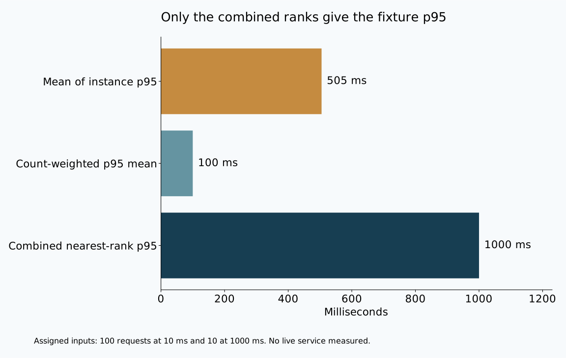
The service p95 in this fixture is 1000 milliseconds. Averaging its two instance p95 values gives 505 milliseconds. Weighting those values by request count gives 100 milliseconds. Neither average is the service percentile, even though both calculations are arithmetically correct.
The inputs are deliberately simple: instance A has 100 requests at 10 milliseconds each, and instance B has 10 requests at 1000 milliseconds each. The executed calculation uses the nearest-rank definition of p95. It orders all observations and selects position ceil(0.95 × count), with positions counted from one.
These are assigned observations, not measurements from a Dreamtsoft deployment. Their purpose is to expose what is lost when a dashboard combines percentile values instead of the underlying distributions. The 110-row input file lets a reader reproduce every result without a monitoring service.
Calculate the rank before choosing an aggregation
For the combined 110 requests, the selected rank is 105. The first 100 ordered observations are 10 milliseconds. Positions 101 through 110 are 1000 milliseconds. Position 105 therefore returns 1000 milliseconds.
Instance A's p95 is 10 milliseconds, and instance B's is 1000 milliseconds. Their unweighted average is (10 + 1000) / 2 = 505. Their request-count-weighted average is (100 × 10 + 10 × 1000) / 110 = 100. Weighting changes which instance contributes more to the arithmetic, but it cannot reconstruct the positions discarded by each instance's percentile calculation.
| Calculation | Result in milliseconds | Question it actually answers |
|---|---|---|
| A p95 | 10 | A's selected latency rank |
| B p95 | 1000 | B's selected latency rank |
| Mean of instance p95 values | 505 | Average of two summary numbers |
| Count-weighted mean of p95 values | 100 | Weighted average of those summaries |
| p95 of all 110 observations | 1000 | Selected rank of the combined requests |
The weighted result happens to equal the mean request latency in this constructed dataset because every request on each instance has identical latency. That coincidence does not make it a percentile. With a distribution of values inside each instance, a weighted average of instance p95 values generally does not even reconstruct the overall mean.
Percentile algorithms can differ on small datasets. State the definition when publishing an exact fixture result, and check the estimator used by the production tool. This example selects an observed value by nearest rank. It does not interpolate between neighboring values or between histogram buckets.
The percentile can move sharply while traffic changes slightly
Keep A's 100 fast requests fixed and vary the number of 1000-millisecond requests on B. With five slow requests, the total is 105 and the selected p95 rank is 100, so the result is still 10 milliseconds. With six slow requests, the total is 106 and rank 101 selects 1000 milliseconds.
That jump follows directly from the chosen distribution and rank definition. It does not mean that every request became 100 times slower between the two cases. The slow-request share crossed the point that determines the selected rank. A percentile dashboard alone cannot tell whether that happened because one route slowed down, traffic shifted toward a slow route or the measurement population changed.
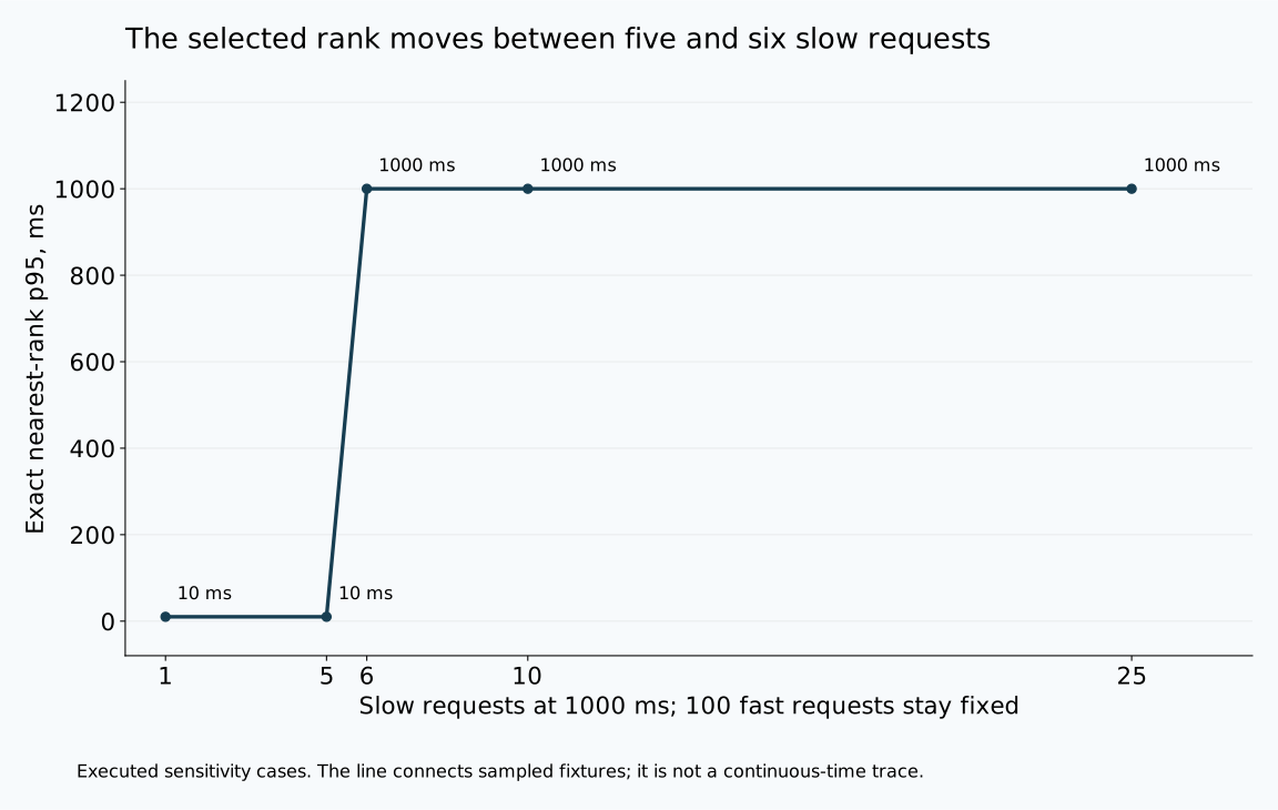
The results file includes five sensitivity cases with 1, 5, 6, 10 and 25 slow requests. Read their counts alongside their p95 values. Two windows can share the same percentile while containing very different numbers of affected requests.
For operational review, retain the request count and the relevant distribution, then examine route or service boundaries that have a meaningful interpretation. Creating a label for every request or customer is not necessary to understand the population shift. The metric-cardinality example examines the cost of using unbounded identities as metric dimensions.
Combine distributions over the same population and interval
Prometheus's histogram and summary guidance explains why precomputed summary quantiles cannot be aggregated across instances, while histogram observations can support aggregation before quantile estimation. The useful ordering is to combine compatible distributions first and estimate the requested quantile afterward.
"Compatible" matters. Check that the series represent the same latency unit, measurement boundary and time interval. A server request duration and a database query duration answer different questions even if both are measured in seconds. Summing distributions from overlapping measurement points may count the same user operation more than once.
Classic histogram buckets also need compatible boundaries for a meaningful combined bucket population. The resulting quantile is an estimate based on the bucket distribution, not the exact nearest-rank result from our raw observations. Native histogram behavior and query syntax depend on the actual monitoring setup; this fixture does not exercise either representation.
Time aggregation requires the same care. An average of hourly p95 values does not produce the day's p95. If the question concerns all requests in a day, obtain a distribution for that population and interval. If the question is instead how often an hourly p95 exceeded a threshold, keep that explicitly different measure and label it accordingly.
Review the dashboard with a counterexample it must explain
A dashboard review can use this dataset as a reasoning check. Ask where the raw distribution or bucket counts enter the calculation, which labels are combined and whether the output is a percentile estimate or an average of percentile series. The formula should explain why the exact fixture's combined p95 is 1000 milliseconds.
Do not require a bucket-based estimator to equal the exact raw-data result without examining its bucket layout and interpolation. Instead, verify that its estimated value has a documented relationship to the chosen buckets. A discrepancy can reveal an estimator limitation rather than an implementation bug.
Finally, choose the user-facing reliability question before selecting p95. A latency objective expressed as a proportion of requests below a threshold can be evaluated through good and total request counts over its defined interval. The SLO burn-rate example addresses that ratio-based question. It should not inherit a percentile average simply because that number already exists on a dashboard.
The local script proves a narrow point with complete input data: neither ordinary nor count-weighted averaging recovers the combined percentile. A production review still needs to establish what was measured, how it was grouped and which estimator generated the displayed number.
Sources
Documentation checked .
Dreamtsoft Editorial
Request weighting sounds persuasive until the raw ordered observations are beside it. The selected combined rank is information that the instance percentile summaries no longer contain.
Dreamtsoft Editorial
The sensitivity cases make a useful dashboard review exercise. A percentile jump can follow a change in the share of slow requests without every request becoming slower.
Dreamtsoft Editorial
The nearest-rank definition belongs beside the fixture result. Another estimator may produce a different small-sample value without making the arithmetic in this example wrong.
Dreamtsoft Editorial
A service dashboard should state which requests enter the distribution. Mixing a database-call duration with an end-to-end request duration changes the measured population.
Dreamtsoft Editorial
The same aggregation question applies across time windows. An average of hourly percentile values does not recover the distribution of all requests during the day.
Dreamtsoft Editorial
For a histogram-based reproduction, inspect the bucket boundaries before comparing the estimate with the exact raw-data result. The two calculations retain different information.
Dreamtsoft Editorial
Keeping counts beside the percentile helps distinguish identical tail values with different numbers of affected requests. That context matters when comparing two incident windows.
Dreamtsoft Editorial
A threshold-based latency objective asks a different question from p95. The review should identify the intended good-request rule before reusing an existing dashboard number.