

The same capacity can produce different waits
A noisy neighbor is a tenant whose use of shared resources degrades another tenant's experience. In background processing, the symptom may be an export that stays pending while another customer imports a large file. The affected customer did nothing unusual. Its jobs simply entered a queue behind work that already occupied the workers.
Microsoft frames the noisy neighbor problem as resource governance. That framing matters here: storing tenant data separately would not change which background task receives the next worker slot. This experiment isolates that scheduling decision.
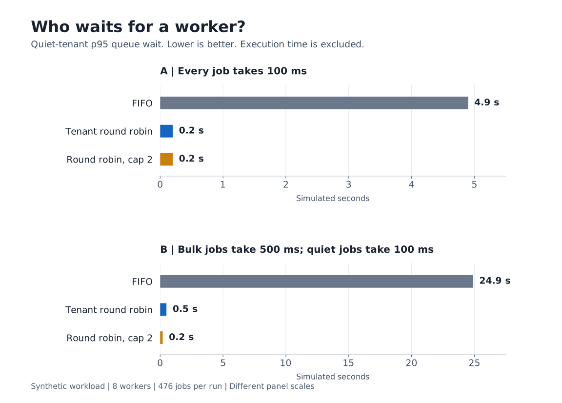
| Bulk job duration | Policy | p95 queue wait | Maximum queue wait |
|---|---|---|---|
| 100 ms | FIFO | 4,900 ms | 5,000 ms |
| 100 ms | Tenant round robin | 200 ms | 200 ms |
| 100 ms | Round robin, cap 2 | 200 ms | 200 ms |
| 500 ms | FIFO | 24,900 ms | 25,000 ms |
| 500 ms | Tenant round robin | 500 ms | 500 ms |
| 500 ms | Round robin, cap 2 | 200 ms | 300 ms |
Every policy completed the same jobs.
The differences came from when those jobs started. In the first workload, all jobs needed the same execution time. In the second, only the bulk tenant's jobs became slower. Round robin still helped the quiet tenants, but its p95 wait rose to 500 ms because running jobs could not be interrupted.
These are results from a deterministic model, not measurements of a deployed service. They support a narrow conclusion: with this arrival pattern and these execution times, changing admission order redistributed delay. They do not predict the latency of your application.
How the experiment was run
We wrote a discrete-event simulator that advances an integer clock to the next arrival or completion. A worker executes one job at a time. There is no sleeping, network traffic or random sampling. Each policy receives an identical copy of the workload, making the scheduling rule the only change within each scenario.
Method
- Workers
- 8 identical slots
- Tenant population
- 1 bulk tenant and 19 quiet tenants
- Bulk arrival
- 400 jobs at simulated time 0
- Quiet arrivals
- Each quiet tenant sends 1 job at 200, 600, 1,000 and 1,400 ms
- Service times
- Quiet jobs: 100 ms; bulk jobs: 100 ms or 500 ms
- Percentile rule
- Nearest rank: the 73rd sorted waiting time out of 76 quiet jobs
- Tie handling
- Completions first, arrivals second, dispatch third; simultaneous arrivals use ascending job ID
- Exclusions
- None; all 476 jobs must complete
The quiet cohort is a fixed label in the input. It is not inferred from outcomes, and no inconvenient tenant is removed from the percentile. Queue wait means start time minus arrival time. Completion latency also includes service time. For these quiet jobs, it is 100 ms longer. Comparing one metric with the other would change the meaning of the result.
| Policy | Next job selection | Treatment of unused capacity |
|---|---|---|
| FIFO | Take the oldest arrived job from one global queue. | Dispatch whenever any job is waiting. |
| Tenant round robin | Rotate through tenant IDs and take one waiting job from the next nonempty tenant queue. | Skip empty queues; a lone active tenant can fill all 8 slots. |
| Capped round robin | Use the same rotation, but skip tenants with 2 jobs already running. | The cap is hard. Slots stay idle when no tenant is eligible. |
Results and verification
Each run writes a start and finish time for every job. An independent sweep over those intervals checks worker capacity and the per-tenant cap. Small fixtures with manually calculable answers check FIFO order, round-robin order, idle periods and the percentile rule. The script repeats every run and requires identical output. All 476 jobs completed in each run.
Limits
- The model excludes broker delivery, polling and scheduling overhead. It cannot compare message-queue products.
- All tasks succeed. Retries, crashes, database locks and connection limits are absent.
- The input contains one finite burst. Sustained overload and several competing bulk tenants need separate experiments.
- Queues are unbounded and workers never preempt a running job. Neither assumption should silently become a production requirement.
The workload was designed to expose a scheduling trade-off. It is not a random sample of SaaS traffic. Treat the output as a testable example, then replace its assumptions with measurements from the system you operate.
Put the tenant boundary before the worker pool
A scheduling policy needs a trustworthy answer to one question: whose work is this? Attach the tenant identity when the application accepts the operation, and carry it through the job record. Derive that identity from authenticated application context. Accepting an arbitrary tenant label from the payload would let callers choose which budget they consume.
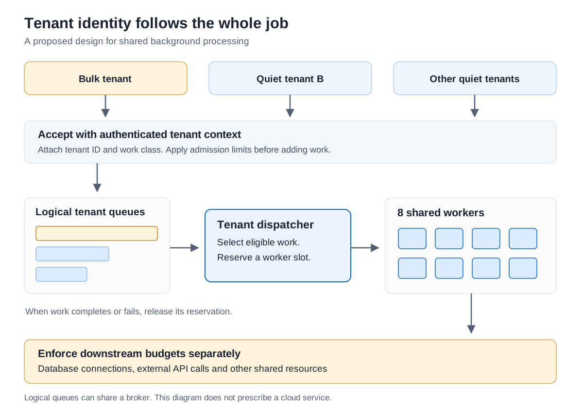
- Admission: identify the tenant and work class, then decide whether to accept, defer or reject the operation.
- Logical queues: preserve the tenant identity while jobs wait. Separate logical queues do not require separate deployed brokers.
- Dispatch: choose an eligible tenant, reserve a worker slot and record the start time.
- Execution: apply separate budgets to database connections and external calls, then record the outcome and release reservations.
A shared dispatcher can coordinate separate tenant queues, or a broker can expose a fairness feature. The application still needs to know the feature's actual semantics. Amazon SQS fair queues, for example, use MessageGroupId as a tenant identifier on standard queues and prioritize other tenants when one has disproportionately many in-flight messages. AWS states that this does not enforce message ordering or impose a per-tenant consumption-rate limit.
Our round-robin algorithm does not reproduce that managed service. The distinction affects design: a fairness feature is not automatically a hard concurrency cap, and a tenant label is not automatically an ordering guarantee. Verify both behaviors before relying on them.
For an integration-heavy product, trace the full path from accepted API request to completed background operation. Dreamtsoft's REST API integrations overview is a separate entry point for its integration scope. The architecture illustrated here is a general design example.
A hard cap protects capacity by leaving some of it unused
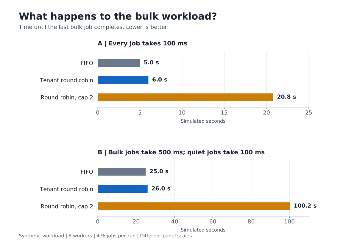
The quiet-tenant chart makes the cap look attractive. The bulk completion chart shows the other half of the decision. A tenant with a large legitimate import also has a user waiting for the result. Record that user's completion target alongside the targets for the smaller jobs.
| Scenario | Policy | Bulk finished at | Worker utilization |
|---|---|---|---|
| Equal jobs | FIFO | 5.0 s | 99.17% |
| Equal jobs | Tenant round robin | 6.0 s | 99.17% |
| Equal jobs | Round robin, cap 2 | 20.8 s | 28.61% |
| Slow bulk jobs | FIFO | 25.0 s | 99.81% |
| Slow bulk jobs | Tenant round robin | 26.0 s | 99.81% |
| Slow bulk jobs | Round robin, cap 2 | 100.2 s | 25.90% |
Utilization here is total simulated service time divided by 8 times the interval from time 0 until the last completion. It describes occupied worker slots, not CPU usage or infrastructure cost. A worker waiting on a real database might occupy a slot while consuming little CPU.
Uncapped round robin finished the entire workload at the same time as FIFO in both scenarios: 6.0 seconds for equal jobs and 26.0 seconds for slow bulk jobs. It moved some bulk work later so quiet jobs could start earlier.
The result does not show a throughput increase. It shows a different allocation of a fixed capacity.
After the quiet jobs drain, the hard cap still permits only 2 bulk jobs to run. The other slots cannot help. A policy that lends unused capacity could avoid some of that delay, but would need a rule for taking the capacity back when another tenant arrives. That lending policy was not tested here.
Round robin distributes dispatch opportunities by job count. When one job occupies a worker much longer than another, equal turns do not imply equal resource time. Google's Handling Overload explains why request counts can be poor proxies for resource cost. For mixed workloads, consider separate work classes or measured resource budgets before assuming a count-based policy provides the desired isolation.
Choose the isolation boundary that matches the bottleneck
A slow queue can be the first visible symptom of a bottleneck elsewhere. If each worker opens a database connection and holds it for the whole job, admitting tenants fairly still leaves them competing for that connection pool. Adding queues would change organization without changing the scarce resource.
| Observed condition | Control to evaluate | What remains shared |
|---|---|---|
| Short tasks wait behind a bulk backlog. | Tenant-aware dispatch across the shared worker pool. | Workers and every downstream dependency. |
| A tenant occupies many slots with long tasks. | Per-tenant concurrency cap or a separate work class. | Storage capacity and external-service limits. |
| A tenant exhausts database connections. | A connection budget at the database access boundary. | Query execution resources and database locks. |
| Workloads require separate failure domains. | Dedicated worker pools or deployment partitions. | Any dependency that was left common. |
| Many tenants exceed total available capacity together. | Admission limits and capacity planning against aggregate demand. | The physical capacity ceiling until it changes. |
Microsoft's multitenant messaging guidance describes shared, dedicated and hybrid arrangements. It also notes that dedicated messaging can leave other shared components exposed. Use that distinction when evaluating a platform as a service: identify what the provider isolates and what your application continues to share.
Security isolation needs its own review. A separate logical queue may help a scheduler recognize tenants without preventing a worker from reading another tenant's data. Authorization, credentials and data-access rules must remain effective independently of scheduling. Keep those checks in the job execution path, including retries and administrative replay.
Business priority is another input. A short job is not necessarily important, and a long job is not necessarily optional. Define work classes using the operation's consequence and deadline. A foreground confirmation and a scheduled bulk export can legitimately need different admission rules even when they belong to the same customer.
Before documenting a queue policy for a workflow automation use case, specify what happens when the relevant limit is reached. A caller needs a distinguishable outcome: accepted for later processing, rejected with a retry instruction or completed. An indefinitely pending task gives the user no reliable next action.
Test both the waiting customer and the bulk customer
Start with a trace you can explain. A global average can conceal the exact cohort that needs protection, while a quiet-tenant percentile can conceal a bulk workload that has stopped making acceptable progress. Compare both views for the same interval and keep the input trace fixed between policies.
- Record arrival, start and finish timestamps together with the tenant ID, work class and outcome. Keep queue waiting time separate from service time.
- Replay the same trace with the proposed policy and the current policy. Keep worker count and downstream budgets unchanged for this comparison.
- Inspect each tenant's waiting-time distribution and completion rate. Keep rejected, timed-out and failed jobs in the accounting instead of calculating latency only for successful work.
- Check the bulk workload's completion deadline. A policy that protects quiet jobs by making a legitimate import impractically slow needs a different budget or work class.
- Repeat with long jobs, coincident bursts and a downstream slowdown. Then interrupt a worker to test whether its reservations expire and work can resume.
Choose pass criteria before running the test. The 200 ms result in this model is not a sensible default target for every SaaS application. A target should describe a user-visible requirement, the traffic conditions under which it applies and the response when those conditions are exceeded.
| Signal | What it helps diagnose |
|---|---|
| Queue wait by tenant and work class | Which accepted work waits for admission. |
| Service time and downstream wait | Whether execution or a dependency became slower. |
| In-flight jobs per tenant | Whether reservations enforce the intended cap. |
| Bulk completion time | Whether large workloads still finish acceptably. |
| Rejected and expired jobs | Whether apparent latency improved by dropping work. |
| Worker occupancy alongside dependency usage | Whether slots are busy doing useful work or waiting elsewhere. |
Retries deserve a separate workload. Give replayed work the same tenant identity and an explicit attempt budget. Otherwise an unhealthy integration can return repeatedly as apparently new work. Google's overload guidance discusses client-side throttling because even rejected requests consume resources. Increasing rejection traffic without slowing senders can create another bottleneck.
For a rollout, retain a way to compare the new scheduler with the previous behavior and to revert its configuration. Treat the dispatcher as production code with its own availability requirements. A lost reservation or a tenant queue omitted from rotation can strand work even when every worker is healthy.
Reproduce the numbers, then change the assumptions
The experiment uses only the Python standard library. Download the simulation source, save it as queue_simulation.py and run it locally. The file is served as text so you can inspect it before execution. It creates a summary and a complete job trace in the output directory you choose.
python3 queue_simulation.py --out resultsThe reference results JSON records every assumption and all 6 summaries. The job trace CSV contains 2,856 rows, one per job per run. For one scenario and policy, select the 76 rows whose tenant is not 0, sort wait_ms and read the 73rd value. That independently reconstructs the reported p95.
For bulk completion, select tenant 0 and take the largest finish_ms. To reconstruct worker utilization, sum service_ms across all jobs in that run, then divide by 8 multiplied by the largest finish_ms. Multiply by 100 for a percentage. Preserve scenario and policy filters throughout. Combining runs would produce a meaningless denominator.
Change one assumption at a time. Begin with the bulk burst size, then its job duration. Move a quiet arrival inside a long-running batch to see the effect of nonpreemption. After those checks, add a second bulk tenant or vary service times using a trace from your application. Keep any customer identifiers and payloads out of shared experiment files.
A production candidate also needs behavior that this reference model deliberately omits: bounded backlog, durable job state, reservation expiry and clear failure outcomes. Write those requirements beside the policy before implementation. The useful deliverable is a dispatch rule with a reproducible workload and explicit limits on what its results establish.
Sources
Documentation checked .